
How an Operational Amplifier Actually Works
The two inputs are not equal. They are driven close together, and five things can stop that happening.
- Lesson 1 of 10
- Intermediate
Almost every explanation of an operational amplifier starts with two rules: no current flows into the inputs, and the two inputs are at the same voltage. The rules work. You can design a great deal of real hardware with nothing else.
The trouble is that the second rule is not a property of the amplifier. It is a result produced by the circuit around it, and the circuit can stop producing it. When that happens the arithmetic goes on being correct while the hardware goes on being wrong, which is a difficult combination to debug if you believe the inputs are equal by law.
Quick answer. An op amp amplifies the difference between its two inputs by an enormous factor. On its own that makes it useless: a millivolt of difference would slam the output into a supply rail. Negative feedback fixes this by returning part of the output to the inverting input, so the output settles wherever it has to in order to make the difference between the inputs very small. The inputs end up nearly equal because the output drove them there, not because the amplifier holds them together.
What the part actually is
Strip away the triangle and an op amp is a differential amplifier with a very large voltage gain and a single-ended output. It looks at the voltage between its two inputs, multiplies it, and drives the output with the result. The multiplier is called open-loop gain, written AOL, and on a precision part at DC it is commonly 100,000 or more.
Put numbers on that. With an open-loop gain of 100,000 and the output sitting at 2.38 V, the voltage difference between the inputs is:
VID = VOUT / AOL = 2.38 / 100 000 = 23.8 µVTwenty-three microvolts. Not zero, and for many circuits not small enough to ignore, but small enough that calling the inputs equal is a reasonable working approximation. This is the honest form of the rule, and it carries its own caveat with it: the approximation is only as good as AOL, and AOL is not a constant.
Why negative feedback does the work
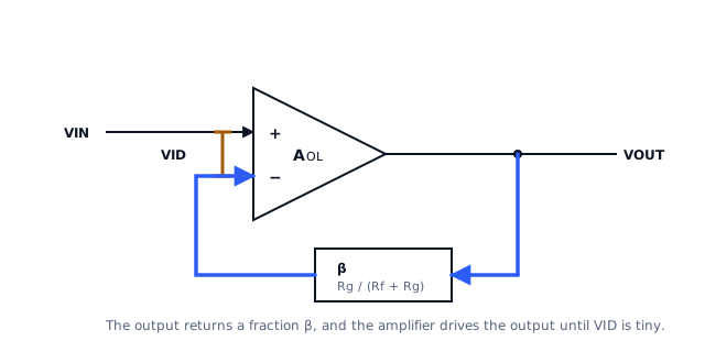
Follow the loop in the figure. The output passes through a resistor divider, and a fraction of it arrives back at the inverting input. If the output is too low, the inverting input is too low, the difference between the inputs is positive, and the amplifier drives the output up. If the output overshoots, the difference reverses and the amplifier drives it back down.
The output therefore comes to rest at the value that makes the difference nearly zero. It is a servo, and like any servo it is the loop that holds the error small, not the actuator.
Two consequences follow immediately, and both are more useful than the rules they replace.
- The gain is set by the divider, not by the amplifier. If the divider
returns one part in 119 of the output, the output must be 119 times the input to balance the loop. Change the resistors and you change the gain. Change the amplifier and, at DC, you mostly do not.
- The amplifier's own gain only has to be large enough. It does not have
to be accurate, stable with temperature, or the same part to part. All of that inaccuracy is divided down by the loop, which is the whole reason the configuration is worth using.
Where the error actually lives
The gap between the inputs is the error signal of the servo, and it is inversely proportional to how much loop gain is available. At DC, with AOL of 100,000, the gap is 23.8 µV in our example. But AOL falls as frequency rises. If at some frequency of interest the open-loop gain has dropped to 1,000, the same 2.38 V output requires:
VID = 2.38 / 1 000 = 2.38 mVA hundred times worse, from the same amplifier in the same circuit, with nothing changed but frequency. The closed-loop gain error grows in step with it. This single relationship is why an op-amp circuit that is accurate at DC can be visibly inaccurate at a few kilohertz, and it is the subject of the gain-bandwidth lesson later in this course.
Five ways the assumption stops being true
The near-equality of the inputs is a conclusion, and conclusions have premises. These are the five premises that fail in practice.
- The output has run out of range. If the required output is beyond what
the supply rails and the output stage allow, the loop cannot balance. The output sits as close as it can get and the inputs separate by whatever is left over. This is saturation, and it is the only one of the five that is usually obvious.
- There is not enough gain left at this frequency. As above. Nothing
dramatic happens, the error just grows smoothly, which is exactly why it gets missed.
- The output cannot move fast enough. During a fast transition the output
may be limited by its maximum rate of change rather than by gain. While that lasts, the loop is effectively open and the inputs can be volts apart. This is slew-rate limiting, and it has its own lesson.
- An input is outside its valid common-mode range. The input stage is
built from transistors that need some headroom to the rails. Take the inputs outside the range the datasheet specifies and the stage stops behaving like a clean differential amplifier, even though the output may still be sitting in a perfectly plausible place.
- The feedback is not actually negative at the frequency that matters.
Enough phase lag around the loop and the correction arrives late enough to make matters worse. The circuit rings, or oscillates, and the quiet assumption that the inputs are together is the first casualty.
Each of those gets a lesson of its own. What matters here is that they are not exotic failures. Four of the five produce a circuit that looks like it is working.
Ideal and real, side by side
| Property | Ideal model | What a real part does |
|---|---|---|
| Open-loop gain | infinite | large at DC, falling with frequency |
| Input difference | zero | output divided by the gain available |
| Input current | zero | picoamps to microamps, depending on technology |
| Input offset | none | a fixed error added to the real difference |
| Input range | any voltage | a window set by the supplies and the input stage |
| Output range | rail to rail | short of each rail by an amount the load decides |
| Output speed | instant | limited by both bandwidth and slew rate |
| Stable? | always | depends on the loop, including the load |
The right way to read that table is not as a list of disappointments. It is a list of the questions to ask about a candidate part, and the rest of this course is those questions in order.
What comes next
Lesson 2 builds the two configurations this whole course uses, the inverting and the non-inverting stage, with the same pair of resistors in both, and shows the three things that differ which the gain equations do not mention.
An op amp also needs its supply pins decoupled to behave like the device in its datasheet, which is a separate subject handled in the decoupling lesson of the power integrity course.
Sources and further reading
- Texas Instruments: Understanding Operational Amplifier Specifications (SLOA011) — application report, how the datasheet parameters relate to circuit behaviour.
- Texas Instruments: AN-20 An Applications Guide for Op Amps (SNOA621) — application report, the classic treatment of feedback configurations and their error terms.
- Microchip: AN722 Operational Amplifier Topologies and DC Specifications — application note, the DC specifications and what each one costs you.
- Texas Instruments: Ramping Up on Slew Rate (SLOA332) — application note, on why the input difference must be non-zero for the output to move at all.