
Gain-Bandwidth Product: Why Op-Amp Gain Falls with Frequency
A gain of 119 from a 1 MHz part leaves you 8.4 kHz, and nothing on the schematic says so.
- Lesson 3 of 10
- Intermediate
A datasheet says 1 MHz. The circuit is built, the gain is right, and at 10 kHz the output is visibly smaller than it should be. Nothing is broken. The 1 MHz was never available at the gain you asked for.
Quick answer. Gain-bandwidth product is the open-loop gain of the amplifier multiplied by the frequency at which it is measured, and for most general-purpose op amps that product is roughly constant over a wide range of frequencies. Divide it by your circuit's noise gain and you get the approximate frequency at which the closed-loop response falls by 3 dB. A 1 MHz part in a stage with a noise gain of 119 gives about 8.4 kHz.
Where the number comes from
Open-loop gain is not a single figure. It is enormous at DC, stays there up to some low frequency, and then falls steadily. For a part with a single dominant pole, which describes most internally compensated op amps, it falls at a rate of ten times less gain for every ten times more frequency.
A constant rate of that kind means the product of gain and frequency is constant. That product is the gain-bandwidth product, and it is also, by the same arithmetic, the frequency at which the open-loop gain has fallen to 1.
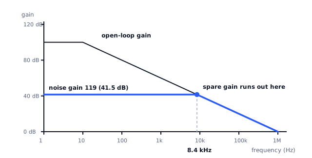
The figure shows the two curves that matter. The falling line is the amplifier's open-loop gain. The horizontal line is your circuit's noise gain, the gain the loop is being asked to provide. Where they meet, the amplifier has exactly as much gain as the circuit demands and no more to spare. Above that frequency the loop is running out of authority and the closed-loop gain follows the open-loop curve down.
That intersection is the closed-loop bandwidth. It is not a separate phenomenon, it is a reading taken off a graph.
Working the number for our front end
Our stage from the previous lesson has a noise gain of 119. Suppose the amplifier is specified at a gain-bandwidth product of 1 MHz.
f−3dB ≈ GBW / noise gain = 1 000 000 / 119 = 8 403 HzSo 8.40 kHz. For a thermocouple or a load cell that is comfortable. For anything that needs to track a signal at 20 kHz it is a failure, and the failure is quiet: the gain is simply low, with a phase shift that accompanies it, and the circuit looks like it is working.
Notice which gain did the dividing. It is noise gain, not signal gain. Build the inverting version of the same stage, with a signal gain of 118, and you still get 8.40 kHz, because the loop does not know or care which terminal your signal came in through.
If you need more
Three routes, in increasing order of how much they cost you.
Buy more gain-bandwidth. To reach 50 kHz at a noise gain of 119:
GBW ≥ 50 000 × 119 = 5.95 MHzSo you need a part specified at 5.95 MHz or better, which in practice means choosing from a different and usually hungrier family. Gain-bandwidth is paid for in quiescent current more often than in money.
Split the gain across two stages. Two cascaded stages of equal gain multiply to 119 when each has a gain of:
√119 = 10.9Each stage then gets 1 MHz / 10.9 = 91.7 kHz of bandwidth from the same 1 MHz amplifier. The cascade is narrower than either stage, because two responses rolling off together reach −3 dB sooner than one does. For two identical stages the combined −3 dB point is about 0.64 times the single-stage figure:
f−3dB(cascade) ≈ 91 700 × 0.64 = 59.0 kHzStill seven times the single-stage bandwidth, from the same amplifier, at the cost of a second one and a second set of error terms.
Accept less gain and give the work to the converter. Sometimes the honest answer is a gain of 20 and a converter with more bits.
| Noise gain | Bandwidth from a 1 MHz part |
|---|---|
| 1 | 1 MHz |
| 10 | 100 kHz |
| 119 | 8.4 kHz |
| 1000 | 1 kHz |
Where the rule stops being true
Gain-bandwidth product is a good approximation with named limits, and treating it as a law produces confident wrong answers.
- It assumes one dominant pole. Internally compensated general-purpose
parts are designed to behave that way. Decompensated amplifiers, which trade unity-gain stability for more gain-bandwidth, do not, and are only usable above some minimum closed-loop gain stated in the datasheet.
- It does not apply to current-feedback amplifiers at all. In those the
bandwidth is set largely by the feedback resistor, and changing gain by changing Rg barely moves it. Using the GBW rule on one gives nonsense.
- The −3 dB point is not always a clean roll-off. With limited phase
margin the response peaks before it falls, so the amplitude at the −3 dB frequency is reached on the way down from a bump rather than on a smooth curve. That peaking is the same phenomenon as the ringing in the capacitive load lesson.
- The specification has conditions. Gain-bandwidth is measured at a stated
supply voltage, load and temperature, and is typically a typical value rather than a guaranteed minimum. A part at the cold end of its range may not deliver it.
Small signal is not the same as large signal
Everything above describes the small-signal response: what happens to a signal small enough that the amplifier's output is never trying to move faster than it can.
Our front end's full-scale output is 2.38 V, which is not a small signal. At some combination of amplitude and frequency, a completely different limit takes over, one that has nothing to do with gain-bandwidth product and is not predicted by anything in this lesson. The output stops being able to change fast enough.
That is slew rate, and it is next.
Sources and further reading
- Texas Instruments: Operational amplifier gain stability, Part 3: AC gain-error analysis (SLYT383) — journal article, how open-loop gain roll-off turns into closed-loop gain error.
- Texas Instruments: Feedback Plots Define Op Amp AC Performance (SBOA015) — application bulletin, reading bandwidth and stability off the intersection of the two curves.
- Texas Instruments: Understanding Operational Amplifier Specifications (SLOA011) — application report, the conditions attached to the AC specifications.
- Microchip: AN723 Operational Amplifier AC Specifications and Applications — application note, the AC parameters and how they limit a circuit.